
Corn ethanol is not mandated under the RFS. However, 98% of “conventional biofuels” produced in the U.S. and blended into gasoline are derived from corn, thus creating a de facto mandate for corn ethanol. The RFS mandate for conventional biofuels is set to rise from 13.2 billion gallons in 2012 to 15 billion gallons in 2015. With the additional mandate for advanced and cellulosic biofuels, the total blending requirement rises to 36 billion gallons by 2022. The U.S. Environmental Protection Agency (EPA) administers the RFS program and is the only U.S. agency with the authority to waive or delay implementation of volumetric mandates for renewable fuel blending into the gasoline and diesel pools.
In response to concerns over reductions in corn production from the widespread drought, five state governors have petitioned the EPA to either reduce or waive the RFS mandates and nearly 200 members of Congress (from both the Senate and House) have publicly announced their support for a waiver. The EPA announced on August 20, 2012 that it will accept comments for 30 days on the governors’ waiver request. The EPA is expected to act on the requests before November 13, 2012, but the agency’s likely response, if any, is unknown.
Drought throughout much of the U.S. farm belt is expected to severely reduce the 2012 corn crop. The U.S. Department of Agriculture (USDA) in June 2012 predicted a record 14.79 billion bushels of corn for the current harvest, but their forecast was revised down to 10.73 billion bushels in September 2012. The new forecast places the corn harvest at the lowest level since 2006 and 13% below 2011 output. Poor expectations on corn harvests are now setting all time price records with corn rising above $8 per bushel. High corn prices have made ethanol production unprofitable for producers with higher cost structures, and several ethanol plants have been idled or are operating at reduced capacity. Ethanol production has declined from 920,000 bbl/d (barrels per day) in June 2012 to 829,000 bbl/d during the final week of August. The Energy Information Administration (EIA) forecasted in its September Short Term Energy Outlook that production will average 830,000 bbl/d in the second half of 2012 and 870,000 bbl/d during 2013. An 870,000 bbl/d production rate would consume 4.9 billion bushels of corn over one year. The U.S. is a net exporter of ethanol, but imports have declined by 80% since the beginning of the year to 20,000 bbl/d.
Ethanol is currently blended into the gasoline pool at 9.7% concentration and blending volumes plateaued in 2010. But volumetric requirements under the RFS will soon take ethanol past the 10% “blendwall.” EPRINC has calculated that by 2014 the blendwall is likely to be breached. At that time, the gasoline pool will be completely saturated by ethanol at virtually 10% concentration, carryover RINs (renewable identification numbers) will be exhausted, and cost and distribution constraints mean that higher ethanol blends such as E15 and E85 will provide little relief for obligated parties to meet RVOs (renewable volumetric obligation). However, given the potential that U.S. gasoline consumption may continue to decline and that more carryover RINs could be used in the current period to overcome further declines in ethanol production, there is a distinct risk that the blendwall will be breached in 2013.
Obligated parties such as refiners have several means for meeting RFS mandates in 2012 should ethanol production become severely curtailed or blending become uneconomic. There are an estimated 2.4 billion carryover RINs which can be applied towards 2012 RVOs. Ethanol inventories were at 18.7 million barrels (785.4 million gallons) as of the final week of August and some of these inventories could be drawn upon by obligated parties to help meet volumetric blending requirements. Obligated parties face a dilemma if they choose to meet current volumetric obligations through greater use of RINs and existing inventories. This is because ethanol blending is much more costly for obligated parties once the blendwall is reached, and using inventories and RINs now, particularly in a short supply environment, would preclude using them later when they are much more valuable. Any waiver that does not push off the blendwall, perhaps by as much as 2-3 years, will not substantially reduce current blending demand. Unless the blendwall is pushed off by several years, obligated parties will continue to face a strong economic incentive to continue blending ethanol at up to 10% concentration and acquire RINs in the current period to apply to future obligations.
Ethanol producers have called for no revisions in the mandate for blending of conventional biofuels into the transportation fuel supply. The ethanol producers have provided econometric studies and other research that concludes that the mandate has provided large benefits to the U.S. such as enhanced energy security, lower gasoline prices, and the production of a large volume of a DDGS (dried distillers grain with solubles), a by-product for feeding livestock. With regard to ethanol’s effect on gasoline prices, ethanol producers have relied on an RFA (Renewable Fuels Association) sponsored and oft quoted study by the Center for Agriculture and Rural Development that claims the RFS mandate has reduced U.S. gasoline prices by over $1/gallon.
EPRINC’s assessment of the economic and energy security implications of the ethanol mandate concludes that the benefits of the mandate are exaggerated and are now imposing substantial costs on the production of transportation fuels and food. These costs are likely to grow as the percentage of ethanol in the gasoline pool exceeds 10%. The following findings summarize the main conclusions of the EPRINC assessment.
EPRINC’s findings are as follows:
-
A near term waiver of blending requirements (6 months to 1 year) would have little effect on corn demand for the production of ethanol. Obligated parties would still have to plan for RVO compliance once the waiver ends. Blending would still have to occur at high levels now, as obligated parties would want to acquire RINs to prepare for the high (and future) cost of crossing the blendwall. Refiners will also need time to adjust their gasoline yields in response to lower ethanol production. A longer term waiver (2-3 years) at some level at or below the blendwall would allow for a proper assessment of the nation’s crop situation, provide end-users with a stable planning environment, and permit refining operations to adjust fuel output. Such a waiver would likely reduce corn prices, providing economic benefits in the form of feed and food prices, and would reduce the risk of a price spike in gasoline as obligated parties begin blending ethanol at levels above 10% of the gasoline pool.
-
There are no low-cost solutions for marketing renewable fuels into the transportation fuel supply in the near-term at levels above 10% of the gasoline pool. So called higher ethanol blend options, such as E85 (70-85% ethanol blends for flex fuel vehicles) have failed to achieve market success due to their high cost, poorer mileage performance relative to gasoline, and lack of availability. EPA has recently approved E15 for model year 2001 and newer light duty vehicles. E15, however, faces a large number of infrastructure, liability, and cost issues, all of which will limit widespread adoption. Auto manufacturers have not provided warranties for non-flex fuel vehicles using so-called E15 blends.
-
The energy security and cost savings benefits from ethanol have been exaggerated. Ethanol did not reduce gasoline prices by more than $1/ gal in 2011 as was concluded in the oft quoted study from the Center for Agricultural and Rural Development at Iowa State University (CARD). Extensive independent econometric research and EPRINC cost-based models conclude that ethanol had little or no effect on the price of gasoline.
-
Even if ethanol blending were determined strictly by cost and market conditions, total blending would be unlikely to fall below 400,000 bbl/d from current blending volumes of around 800,000 bbl/d. Ethanol blending at the lower level would continue because ethanol remains a valuable blending component to meet octane requirements and other fuel specifications required by EPA. Higher blending levels would occur depending upon cost and market conditions.
-
Fuel adjustments to reductions in ethanol blending are both low cost and technically achievable given time. A reduction in ethanol blending could be made up through relatively small yield adjustments at U.S. refining plants. For example, if U.S. ethanol blending declined to 400,000 bbl/d, U.S. crude oil refiners could make up the volume through yield adjustments of less than 2%, well within technical and historical performance levels of the past decade.
-
By-product production of feed from ethanol production, DDGS, has not substantially lowered the cost of raising livestock in the United States. The ethanol industry purchases approximately 40% of the U.S. corn crop and is the largest purchaser of corn in the United States. Even when DDGS volumes are returned to the livestock feed supply chain, 30% of U.S. corn production is consumed for fuel production. DDGS prices are directly correlated to corn prices; despite the rapid growth of DDGS production resulting from the boom in corn for ethanol, DDGS supply growth has come at the expense of existing feeds such as corn and soy. Twenty percent of the two most widely planted crops in the U.S., corn and soy, went to biofuels production during the 2011/2012 crop year.
-
The RFS’ volumetric mandates have created inelastic demand for ethanol. Many supporters of the blending mandate have claimed that the program has substantial flexibility since it permits obligated parties to use RINs in a subsequent year or even carry a deficit into the next year. However, the use of carryover RINs, or even carrying a deficit, is of limited value. RINs expire one year after the year in which they are generated and deficits can only be carried over for one year. The supply of carryover RINs will quickly go to zero as obligated parties cross the blendwall. Surplus RINs are needed in the prompt period to offset physical blending below RFS mandated volumes. In 2013 mandated conventional ethanol volumes will surpass 10% of the gasoline pool. Cellulosic and advanced ethanol mandates provide further volumetric requirements. Whatever flexibility is contained in the mandated program disappears when it becomes uneconomic to blend above the RVO on an ongoing basis.
-
A multi-year waiver of both the ethanol and biodiesel mandates would free millions of acres of land for food and livestock uses, even after accounting for a decline in DDGS production. As previously stated, a full and long-term waiver of the RFS would not reduce ethanol use to below 400,000 bbl/d. Current biodiesel production, however, would be almost entirely eliminated. More importantly, a multi-year waiver could free over 18 million acres of existing farm land for the production of crops to meet market needs for food, livestock feed, exports, or fuel.
-
Despite the droughts and record prices for corn and other crops, the RFS has ensured that billions of bushels of corn and soy are set to be converted to fuels which offset less than 5% of the nation’s petroleum fuel supply. The U.S. refining industry could make up the loss of all biodiesel and 400,000 bbl/d of ethanol production by adjusting gasoline yields within their historical 10 year range while remaining a net exporter of distillate fuel. The additional fuel production from refiners would require both adequate time to make the adjustments and an expectation that government policy would not impose long-term uneconomic blending requirements, i.e., blending at levels above 10% of the gasoline pool. As stated above, EPRINC’s assessment is that ethanol blending would continue at or above 400,000 b/d even in an environment free of blending mandates.
II. The Value of Biofuels in the Gasoline Pool
U.S. government officials, including Secretary of Agriculture Tom Vilsack, representatives of the Renewable Fuels Association (RFA), and other supporters of expanded mandates for the use of renewable fuels in the transportation sector have argued that the growth in ethanol blending spurred by the RFS has contributed to large reductions in the price of gasoline. These conclusions were taken from a series of studies from the Center for Agricultural and Rural Development at Iowa State University (CARD). The studies concluded that ethanol use had reduced U.S. gasoline prices by approximately $0.89/gallon in 2010 and $1.09 per gallon in 2011. The results of the study were also circulated widely among members of Congress and were part of an extensive advertising program undertaken by RFA.
The authors of the studies undertook a series of econometric calculations evaluating how the U.S. refining sector and gasoline prices would adjust if growth in the use of ethanol in the transportation fuels sector were constrained. The studies evaluated the consequences of limiting ethanol use across several time periods, but most notable were the consequences of constrained blending between January 2000 and December 2010. The authors state in their most recent report, issued in May:
“We update the findings of the impact of ethanol production on U.S. and regional gasoline markets as reported previously in Du and Hayes (2009 and 2011), by extending the data to December 2011. The results indicate that over the period of January 2000 to December 2011, the growth in ethanol production reduced wholesale gasoline prices by $0.29 per gallon on average across all regions. The Midwest region experienced the biggest negative impact of $0.45/gallon, while the regions of East Coast, West Coast, and Gulf Coast experienced negative impacts of similar magnitudes around $0.20/gallon. Based on the data of 2011 only, the marginal impacts on gasoline prices are found to be substantially higher given the increasing ethanol production and higher crude oil prices. The average affect across all regions increases to $1.09/gallon and the regional impact ranges from $0.73/gallon in the Gulf Coast to $1.69/gallon in the Midwest.”
Figure 1 below shows trends in ethanol blending in the U.S. gasoline pool between 2000 and 2011. Note that the volumes consumed through 2011 reflect a combination of government mandates and financial incentives, as well as ethanol’s market value at low blending levels. The $0.45/gallon ethanol ‘blender’s credit’ and tariff on ethanol imports expired at the end of 2011. The U.S. is also a net exporter of ethanol.
Figure 1. U.S. Ethanol Consumption

Source: EIA Data
If ethanol blending is constrained to the 2000 level of 1.6 billion gallons as CARD did in their 2011 report, total ethanol blending lost across the entire period averages to approximately 328,000 bbl/d. The averages are higher in the later years. As stated above, the authors concluded that constraining ethanol use to levels used in 2000 would have increased gasoline prices by $0.89/gallon in 2010 and $1.09/gallon in 2011.
Ethanol has considerable value in the refining sector at low volumes because of its value as an oxygenate and its role in meeting octane targets. Given the phase out of the oxygenate MTBE (Methyl Tertiary Butyl Ether) during the past decade due to environmental concerns, ethanol became the natural substitute. Without the RFS mandates ethanol would likely have replaced MTBE on a 1:1 basis and would be blended today at approximately 400,000 bbl/d. Figure 2 below shows change in ethanol and MTBE blending during the MTBE phase-out.
Figure 2. Ethanol and MTBE

Source: EIA Data, chart from and EPRINC report published in the Oil & Gas Journal.
However, ethanol’s role at concentrations above 3-5% of the gasoline pool are largely as a substitute for gasoline, but its value is limited by ethanol’s lower BTU content, and ultimately, by limitations of the U.S. auto fleet to absorb ever higher volumes of ethanol. On a volumetric basis, ethanol is often cheaper than gasoline. When adjusted for energy content, ethanol is generally more expensive than the gasoline.
The econometric model tested by Du and Hayes does not adequately reflect operating conditions in the U.S. refining industry. The calculations undertaken by CARD prohibited any adjustments in refining capacity and then made a series of calculations on the consequences of limiting annual ethanol use to 1.6 billion gallons annually for the 2000-2010 and then 2000-2011 time periods. However, ethanol production has grown by billions of gallons per year and refining capacity grew by 1 mm bbl/d (million barrels per day) from 2000 to 2010 and by 1.2 mm bbl/d from 2000 to 2011. This is enough refining capacity to process over 15 billion gallons of crude annually.
Figure 3. U.S. Operable Refining Capacity

Source: EIA Data
The constraint in ethanol use (in the CARD calculations) and refining capacity leads to a shortage of gasoline and an increase in gasoline imports and prices, measured through a calculation of the “crack spread.” The assessment then calculated the expected increases in crack spreads as a proxy for the likely increase in gasoline prices. However, adjusting yields in product slates, increasing or lowering crude runs, and modifying the capital structure of the refinery are all common adjustments that occur in the industry when blending components are unavailable or their relative prices adjust. The CARD results were also inconsistent with extensive research undertaken by EPRINC using cost based modeling.
This loss in ethanol blending represents an average loss in gasoline production of approximately 328,000 bbl/d across the studied time period. However, since the principal substitute for ethanol is gasoline, the volume needed to make up the loss must be reduced to account for energy content, i.e., ethanol has approximately 33% less energy content than gasoline. As a result, the actual loss is closer 200,000 bbl/d of gasoline equivalent. This volume loss could have been easily and inexpensively made up through adjustments in refinery operations through any combination of the following:
-
Short-term adjustments in the yield of the product slate to produce more gasoline and the reduction of other refined products. A major factor in this shift is that the volumetric mandates in the RFS almost entirely target gasoline supplies. Volumetric bio-diesel requirements comprise less than 10% of the total volumetric requirements, the remainder target gasoline supplies. Therefore, the mandates have reduced demand for gasoline, causing refiners to respond by producing more diesel fuel, but not necessarily reducing crude runs.
-
Processing of crude types with higher natural yields in gasoline.
-
Running more crude in refineries with spare distillation capacity, both in the U.S. and abroad, for example, European refiners could easily expand throughput to produce additional volumes of diesel for their home market and at the same time produce additional volumes of gasoline for the U.S. market. The U.S. has traditionally been a major outlet for excess supplies of European gasoline.
-
Construction of additional capacity at U.S. refiners. This did occur naturally in addition to ethanol growth, but was not included in CARD’s model.
-
Import additional gasoline from Europe. European refiners have been awash in excess gasoline since Europe’s dieselization initiative. Marginally increasing imports would have had little effect on world prices.
Importance of Adjustments to Refinery Operations
An examination of recent shifts in gasoline shows that refiners could have offset the ethanol volumes lost in 2010 and 2011 without processing an additional barrel of crude oil. Because the RFS mandates are so heavily slanted towards substituting ethanol for gasoline supplies, they have given refiners an economic incentive to shift production away from gasoline towards middle distillates such as diesel. Figure 4 shows the changes in yields over the past decade. The shift can be made through a combination of operational shifts at the refinery, including a change in crude oil feedstock, installing additional processing infrastructure such as a cracker or coker, and adjusting catalysts or blending components. Distillate yields have improved at the expense of stagnating gasoline yields (but because refinery capacity has increased, gasoline production has too) and by the installation of processing equipment to upgrade residual fuel oil to higher value products.
Figure 4. U.S. Refinery Yields

Source: EIA Data
If it is assumed that without the RFS mandates ethanol blending would plateau at 400,000 bbl/d, making it a 1:1 substitute for MTBE, rather than reaching slightly over 800,000 bbl/d in 2010 and 2011, the gasoline pool would have been missing approximately 400,000 bbl/d of ethanol during those two years. Adjusting for ethanol’s lower energy content relative to gasoline, the loss is 265,000 bbl/d. U.S. refiners could have overcome this shortage without running a single additional barrel of crude oil by making a remarkably small operational adjustment of their yields – an adjustment well within the 2000 – 2011 gasoline yield range – and the U.S. would still have distillate capacity to support exports in 2012.
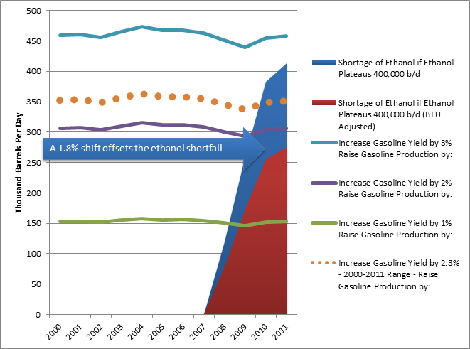
Figure 5 below shows how much additional gasoline would be produced if yields were 1, 2 or 3 percentage points higher, given actual crude oil runs through U.S. refineries for the given year. The orange dotted line shows the increase in gasoline production if yields were raised by 2.3 percentage points – this is the range in which gasoline yields moved during 2000 to 2011. Finally, the red and blue lines are the amount of ethanol that would be missing from the market if ethanol blending was capped at 400,000 bbl/d.
Figure 5. Shifting Refinery Yields to Overcome an Ethanol Shortfall

The chart demonstrates that a 400,000 bbl/d ethanol shortfall could have been covered in 2011 had gasoline yields been just 1.8 percentage points higher, from 45% to 46.8%. A 46.8% gasoline yield is equal to or lower than the gasoline yield during 3 of the past 11 years. It is also well under the 2.3 percentage point range in which yields bounced during 2000 – 2011. Even if ethanol is not adjusted for its lower BTU content, the yield shift required to offset the volumetric shortfall is under 3 percentage points.
If the RFS mandates were completely eliminated, ethanol blending might not decline by as much as 400,000 b/d, and in any case, such an adjustment would take several years. But, blending would certainly drop below RFS mandated levels. Refiners have adjusted to the RFS by optimizing operations to account for 10% ethanol gasoline blends. If given the option, some refiners would eliminate ethanol almost immediately while many others would continue to blend at 10% for probably the next one to three years. This also reinforces the importance of a long-term waiver. Future obligations aside, a temporary waiver of months or even a full year does not give refiners enough time to adjust their operations to reduce ethanol blending.
Blending would remain closer to 10% in summer months so that refiners may obtain a ’1 lb’ RVP (Reid vapor pressure) waiver. Gasoline specifications change during the summer months and a lower RVP of 9 psi (pounds per square inch) is required. By blending 10% ethanol, refiners are granted a waiver of 1 lb. The waiver makes it easier for refiners to meet summer gasoline specifications. E15 will not qualify for a 1 lb waiver.
Figure 5 is not a prediction of what would necessarily occur overnight given the elimination of RFS mandates. However, it illustrates the potential for the refining industry to adjust to more open market conditions and reflects long-term equilibrium demand for ethanol in a mandate free market. The decline in gasoline yields over the past several years were in large part a result of the signal sent by the RFS mandates to refiners which imposed reductions in gasoline output and required ethanol as a replacement. Without the mandate, gasoline yields from U.S. refiners would be higher than they are today.
The ethanol shortfall could be covered without increasing crude oil refinery runs, and therefore without increasing imports. Such a shift might have come at the expense of distillate production and exports. A 1.8 percentage point reduction in distillate yields would have resulted in the loss of 275,000 bbl/d of distillate in both 2010 and 2011. However, this would still have left the U.S. with gross exports of approximately 375,000 bbl/d in 2010 and 575,000 bbl/d in 2011.
It should be noted that Du and Hayes pointed out some of these limitations in their original 2009 study results, the basis for the highly visible 2010 and 2011 updates. But the following statement from the 2009 study is missing in many of the public statements on the contribution of ethanol use in setting gasoline prices.
“These reductions in retail gasoline prices are surprisingly large, especially when one considers that they are calculated at sample mean. The availability of ethanol essentially increased the ”capacity” of the US refinery industry and in doing so prevented some of the dramatic price increases often associated with an industry operating at close to capacity. Because these results are based on capacity, it would be wrong to extrapolate the results to today’s markets. Had we not had ethanol, it seems likely that the crude oil refining industry would be slightly larger today than it actually is, and in the absence of this additional crude oil refining capacity, the impact of eliminating ethanol would be extreme.”
Gasoline prices rise in the CARD calculations because demand can only be met through higher cost production from the existing installed capacity, either in the U.S. or abroad. Additionally, the CARD model does not account for demand rationing. If gasoline prices were $1.09 higher in 2011, a 30% increase which would have sent prices to nearly $5/gallon, certainly demand would have been somewhat curtailed. It should also be remembered that gasoline is a globally traded commodity. The spot price of gasoline in the Gulf Coast is only a few cents per gallon different from the European spot price in Rotterdam. It is unlikely that the loss of 700,000 bbl/d of ethanol under the CARD model, 460,000 bbl/d of gasoline equivalent after BTU adjustment, would have the effect of raising prices $1.09/gallon globally. The CARD report specifies a price impact only in the U.S. market, but the U.S. market is perhaps the most globally integrated fuels market in the world.
A recent study by joint authors from MIT and UC San Diego highlighted the limitations of the econometric approach undertaken in the CARD study. The MIT/UCSD assessment points out that the estimates of reductions in gasoline prices were inconsistent with the basic economics of the industry. The authors of this study concluded that, at best, they were only able to calculate a $0.13/gallon reduction in gasoline prices. In terms of their econometric model results, these conclusions are insignificant or essentially zero. As the authors of the MIT/UCSD study point out, using the same model as the CARD authors, eliminating ethanol use also would have increased natural gas prices by 65 percent and would have caused an increase in U.S. and European unemployment.
Finally, many proponents of expanded ethanol use in the U.S. gasoline pool point out that such use contributes to U.S. energy security through a reduction in oil imports. However, as stated above, ethanol in the U.S. gasoline pool does not reduce oil consumption barrel for barrel. This is because ethanol has fewer BTUs than conventional gasoline. The expansion of ethanol in the U.S. gasoline pool between 2000-2010 is equivalent to approximately 200,000 bbl/d in crude oil savings. The U.S. Energy Information Administration (EIA) shows no substantial benefits in lower import prices to the U.S. in any scenario in which net demand for crude oil or product imports fall by 200,000 bbl/d, barely more than 1% of U.S. petroleum consumption. Such shifts in net demand from EIA show a reduction in the price of gasoline far less than 5 cents a gallon.
Biodiesel – Small Contribution
Biodiesel production is currently on pace to reach 1.5 billion gallons in 2012, equivalent to 100,000 bbl/d. 1 billion gallons of biodiesel are required in 2012 by the RFS. The primary feedstock for biodiesel in the U.S. is soybean oil. During the past three years soybean oil has accounted for 64% to 70% of all U.S. biodiesel production. Biodiesel production and soybean oil’s share of total feedstock are shown in the chart below. Biodiesel production consumed approximately 10% of the 2011/2012 soybean crop.
Figure 6. Biodiesel Production, Sales and Soybean Oil Share

Source: EIA Data, EPRINC Calculation
In 2012, total production of biodiesel will constitute less than 2.5% of the U.S. distillate fuel supply and less than 1% of total petroleum products supplied. If no biodiesel were produced in 2010 and 2011, and ethanol production dropped to 400,000 bbl/d at the expense of distillate yields, as described earlier, the U.S. would have remained a net exporter of distillate. If all biodiesel production is considered part of the distillate pool, net exports would have declined from 375,000 bbl/d to 353,000 bbl/d in 2010 and from 575,000 bbl/d to 512,000 bbl/d in 2011. These volumes are too small to have any impact on global distillate prices and are contributing to distillate exports rather than reducing petroleum based distillate consumption.
III. Why a Temporary or Partial Waiver Will Not Fix Corn Prices or the Blendwall
Obligated parties are currently facing physical constraints in increasing ethanol blending as called for in the RFS. Ethanol is currently blended at 9.7% concentration in the conventional gasoline pool; the effective limit is 10%, referred to as the blendwall. The physical blendwall was reached in mid-2010. Blending volumes then plateaued at an annual rate of approximately 846,000 bbl/d, equivalent to 13 billion gallons per year. As figure 7 below shows, obligated parties blended above mandated levels up until late 2011 (denoted by the blue arrow). By doing so they generated extra RINs which could be carried over to the following year or sold to other obligated parties. Up to 20% of one’s obligation may be carried over and RINs expire at the end of the calendar year following the year in which they were generated.
The RFS mandates continue to grow, yet obligated parties are unable to increase the amount of ethanol they may blend. Obligated parties were, until recently, blending above mandate levels; in 2013 and beyond they will be forced to underblend (denoted by the red arrow), relying on carryover RINs to make up the difference needed to meet RVOs. Conventional ethanol ‘mandates’ will increase from 13.2 billion gallons in 2012 to 15 billion gallons in 2015. Cellulosic and advanced ethanol rise from a combined 1 billion gallons in 2012 to 20 billion gallons in 2022 in addition to the conventional requirements. Cellulosic and advanced ethanol, which includes Brazilian sugarcane ethanol, may also be substituted for corn based ethanol once their respective mandates are met. This provides some flexibility as sugarcane ethanol has a higher RIN value than corn ethanol, but supply is insufficient to offset a large decline in corn ethanol blending.
Figure 7. The Blendwall and RIN Carryover

In 2013 and beyond, obligated parties will use carryover RINs to offset the RVO deficits created by underblending. As RINs are applied to offset underblending, fewer RINs will be eligible for carryover to the following year. The 2.4 billion carryover RINs believed to be eligible for 2012 obligations are needed to avert a blendwall crisis in 2013 and 2014. Any significant decline in 2012 and 2013 blending, due to reduced ethanol production or other factors such a lower gasoline demand, would only serve to advance the date at which carryover RINs are exhausted.
The black box in figure 7 above highlights years in which obligated parties will face a blending deficit: 2013, 2014, and 2015. Assuming constant gasoline demand (EIA projects a slight decline in 2013) and maximum blending of 13 billion gallons per year, the combined RVO deficit over the 2013-2015 period is 4.28 billion gallons (0.83 billion in 2013, 1.43 billion in 2014, and 2.03 billion in 2015). Therefore, when obligated parties transition to a period of blending below mandated levels in late 2012 or early 2013, the current pool of 2.4 billion carryover RINs will only be sufficient to offset RVO deficits until the end of 2014 at the latest. This would require that remaining RINs are eligible to be carried into each of the following years, which will not necessarily be the case. A blendwall crisis is inevitable by 2015, at the latest, absent a change of current policy.
Although current carryover RINs provide near term flexibility in 2012 and 2013, the rise of RVOs over the 10% physical blending limit renders carryover RINs an ineffective tool for mitigating high crop prices or lowering the cost of producing gasoline. A temporary waiver provides little relief because the availability of carryover RINs have a very limited shelf life (one year) and the potential to overblend (and acquire more RINs) continues to decline as the RVO requirements increase.
Under the RFS, EPA may alter or waive volumetric requirements one year at a time. It is unclear if, and how, EPA will respond to the gubernatorial petition. EPA has a large amount of freedom in its ability to modify RFS requirements at the request of petitioners seeking to lower corn and food prices by reducing the ethanol mandates. But the agency is not required to make any changes, and will only do so if it finds that the mandates are creating severe economic harm.
One possible outcome is that EPA will reduce the 2013 mandate. This would theoretically reduce ethanol blending and production, thereby providing the corn and feed markets with much needed breathing room. However, such a waiver will not have its intended effect as long as future RVOs remain unchanged. Obligated parties are already facing a situation in which they cannot meet their RVOs with physical blending and must turn to a limited and shrinking supply of RINs. If the 2013 volumetric requirement were reduced from 13.8 to 10 billion gallons for example, obligated parties would not reduce blending from the current rate of 13 billion gallons per year to 10 billion gallons. Obligated parties would be pressured to continue to blend at 13 billion gallons, using the partial waiver as an opportunity to accrue carryover RINs which could be used to offset 2013 and 2014 deficits, effectively delaying a blendwall crisis by a year or two. Such a situation means the desired loosening of the corn and grain market is not realized.
If obligated parties were to blend at the reduced rate of 10 billion gallons, they would not generate excess RINs and would face the same shortage of RINs in 2014 or 2015 as they do now. Therefore, any potential waiver which seeks to loosen the corn market in the near term must also consider future volumetric ethanol requirements. As EPA does not have the authority to waive multiple years of the RFS (and perhaps does not have the intention), a legislative change may be required to alleviate pressure in the grain market and avert a blendwall crisis.
IV. Ethanol, Biodiesel, DDGS: Food and Fuel
There has been a long running debate on whether ethanol use in the transportation fuels sector is driving up food prices. Some proponents of ethanol use in the transportation sector argue that the U.S. has enormous capacity to expand production of ethanol’s principal feedstock, corn, and can do so with relatively little incremental cost given the availability of land and modern agricultural technology, i.e., many ethanol proponents argue that the supply (cost) curve for expanded corn production does not rise significantly as production increases. Technology, advanced agricultural practices, and the availability of land in the U.S. all suggest that the U.S. can expand agricultural production at relatively low cost, but this view is not universally accepted.
The fundamental question is not whether the U.S. can expand corn production at relatively low cost, or whether using agricultural products in the transportation sector increases food prices, but whether government policy, effectively requiring the use of the nation’s two most widely planted crops, prevents traditional market adjustments to changes in supply and demand and imposes substantial costs on the national economy. The current RFS mandates for ethanol use in gasoline requires that ever higher annual volumes of the fuel be allocated to the transportation sector regardless of the price of corn, or the price of competing fuels and technologies.
Prices play a critical role in the marketplace allowing for, and encouraging, adjustments to changes in relative prices and shifts in technology. These interactions play an important role in producing both fuel and food at the lowest possible cost to consumers. The government mandate prohibits such adjustments even in cases when relative prices shift markedly as is now the case. The RFS’ volumetric mandates have created inelastic demand for ethanol. As built-in flexibilities such as carryover RINs are unworkable long-term solutions, demand adjustments have and will occur by reducing ethanol and grain exports as well as reducing demand among food related end users.
Recent dry weather patterns throughout the agricultural regions of the U.S. are likely to reduce 2012 corn production by approximately 4 billion bushels compared to USDA’s (United States Department of Agriculture) June forecast which was made before the onset of the drought. This represents a nearly 30% decline in crop size. Under the renewable fuels mandate, about 5 billion bushels of 2012 corn production will be allocated to ethanol production. However, the lower corn production forecast is likely to see the percentage of ethanol use raise the amount of corn used for ethanol to 5 billion from 4.25 billion bushels if current ethanol production levels are maintained for 12 months. Production has declined by 160,000 bbl/d since the beginning of the year as high corn prices have caused many ethanol producers to idle production.
Soybeans are the second most widely planted crop in country, after corn. As with corn, the year’s soybean crop is expected to be significantly smaller than previously expected as a result of the drought. In its September crop outlook, USDA forecasted a harvest of 2.63 billion bushels, down from the 3.05 billion bushels predicted in June. This is expected to be the smallest crop in six years and produce the worst yields in 17 years.
Over the past few years, ethanol producers have in fact purchased about 35-40% of the corn crop. They have also generated millions of tons of DDGS which contribute to the feed supply. Ethanol production from corn generates an animal feed component called DDGS (distillers dried grain with solubles), a protein rich byproduct of the ethanol production process that is used as livestock feed. Therefore, not every calorie of corn they purchase ends up as ethanol, a large portion is returned to the food supply. Note, however, as shown in figure 8 DDGS prices closely track the price of corn.
Figure 8. Corn and DDG Prices

Source: USDA Data
Regardless of the reason for corn price increases – a change in planted acres, drought, exports, demand for poultry and livestock feed, demand for high fructose corn syrup and corn flakes, or ethanol demand – rising corn prices raise not only whole corn feed costs but also DDGS costs. Despite huge growth in DDGS production in recent years, DDGS prices remain tied to corn. DDGS growth has largely displaced existing livestock feeds, primarily corn, rather than providing a net contribution; DDGS is the solution to a problem which did not exist before the RFS. Figure 9 below shows the consumption by U.S. livestock of the four most consumed U.S. processed feeds.
Figure 9. Four largest U.S. processed feeds fed, by crop year

Source: USDA Data, see http://www.ers.usda.gov/media/236568/fds11i01_2_.pdf
When one considers that ethanol producers are the largest purchases of corn, at 40% of the annual corn crop in 2011/2012 compared to 14% in 2005/2006, it is clear that ethanol is a major driving force in setting corn prices and more importantly its mandated use means its use remains relatively inelastic.
The RFS Induced Corn Boom
Before the RFS, ethanol was on pace to replace MTBE on a 1:1 basis, which would have put ethanol at 4% of the gasoline pool and require 2 billion bushels of corn annually. But EISA (Energy and Independence Security Act of 2007) went far beyond substituting for MTBE. After EISA was passed in 2007, demand for corn exploded. EISA mandated that 9 billion gallons of ‘renewable’ ethanol be blended in 2008, growing to 15 billion gallons in 2015. By default, this implied corn ethanol. EISA sent a clear signal to the ethanol and agricultural sectors that there would be immediate and rapid demand growth for corn.
Figure 10. Volumetric Biofuel Mandates Under RFS II

Ethanol demand for corn rose from 14% of the 2005/06 harvest, 1.6 billion of 11.1 billion produced bushels, to 40% of the 2010/2011 harvest, or 5 billion of 12.5 billion bushels. The following chart shows corn production and ethanol corn consumption plotted on the left axis, with ethanol’s share of total produced bushels on the right axis.
Figure 11. Corn for Ethanol

Source: USDA Data, EPRINC Calculations
Corn growers responded to the mandates by planting more corn – but not enough. Planted corn acres increased 12.4% from the 2005/2006 crop year to the 2011/2012 crop year. In 2005/2006 81.78 million acres were planted compared to 91.92 million acres in 2011/2012. Yields improved from 2005/2006 through 2009/2010, rising from 147.9 bushels per acre (b/a) to 164.7 b/a, contributing to additional supply growth. But for the past two years yields have declined. The 2011/12 crop yielded just 147.2 b/a and the current 2012/2013 crop is expected to come in at 122.8 b/s, according to USDA’s September outlook.
The 12.4% increase in planted corn acres has not been enough to offset the growth in corn demand for ethanol. This is exacerbated by the recent reversal in yield growth. Ethanol demand for corn in terms of acres planted has grown 26.3 million acres during the past seven years, from 11.4 million acres in 2005/2006 to 37.7 million acres in 2011/2012. After accounting for growth of 10 million planted acres during this period, demand for ethanol still consumes 16 million acres from existing pre-RFS levels. The net result from this overwhelming demand growth is a 210% increase in the price of corn since 2005/2006 and a reduction in corn use by other industries. FarmEcon, LLC pointed out in a July 2012 report that “following the late 2007 increase in the RFS, food price inflation relative to all other goods and services [including energy] accelerated sharply to twice its 2005-2007 rate.” Table 1 below shows the data described above broken down into individual years.
Table 1. Corn Acreage, Yields, Use and Prices
| Crop Year | Alcohol for fuel ethanol | Planted acreage (Million acres) | Production (Million bushels) | Yield per harvested acre (Bushels per acre) | Weighted-average farm price (dollars per bushel) |
| 2005/06 | 1,603.32 | 81.78 | 11,112.19 | 147.90 | 2.00 |
| 2006/07 | 2,119.49 | 78.33 | 10,531.12 | 149.10 | 3.04 |
| 2007/08 | 3,049.21 | 93.53 | 13,037.88 | 150.70 | 4.20 |
| 2008/09 | 3,708.89 | 85.98 | 12,091.65 | 153.90 | 4.06 |
| 2009/10 | 4,591.16 | 86.38 | 13,091.86 | 164.70 | 3.55 |
| 2010/11 | 5,021.21 | 88.19 | 12,446.87 | 152.80 | 5.18 |
| 2011/12 | 5,050.00 | 91.92 | 12,358.41 | 147.20 | 6.20 |
| 05/06 vs 11/12 | 214.97% | 12.40% | 11.21% | -0.47% | 210.00% |
Source: USDA Data, EPRINC calculations.
The USDA chart below shows corn consumption by end user. Consumption growth following the passing of EISA has come at the expense of non-ethanol sectors.
Figure 12. Corn Consumption by Sector

DDGS as a Corn and Soy Substitute
Ethanol refiners use the starch in corn to create fuel alcohol, commonly referred to as ethanol. The ethanol production process generates a protein rich byproduct called DDGS. DDGS is used a feed component for cattle, swine, and poultry feed rations. Approximately 17 pounds of DDGS are generated per bushel of corn processed at an ethanol plant. A typical ethanol plant generates 2.7 gallons of ethanol per bushel of corn. DDGS is primarily a substitute for corn feed but can also substitute for soy meal in certain cases. It may only be fed to livestock in limited quantities and therefore cannot fully replace corn and soy meal, rather it compliments them.
The boom in ethanol production has led to corresponding growth in the DDGS market. DDGS production has grown from 25.92 million short tons (mm st) in 2007/2008 to a projected 42.33 mm st for the 2011-2012 crop year. According to Iowa State University’s DDGS Balance Sheet, in 2011/2012 DDGS substituted for 7.9 million acres of corn (1,159 million bushels of corn equivalent) and 6.09 million acres of soybean production. So although ethanol producers purchased 34 million acres worth of corn last year when yields were 147 bushels per acre, 14 million acres of soy and corn equivalent in the form of DDGS were returned to the feed supply. Sales of DDGS also provide cost recovery for ethanol producers and are an important part of producers’ revenue streams.
The chart below comes from the DDGS Balance Sheet. The amount of DDGS produced is directly proportional to the amount of corn consumed by ethanol plants, although quality may vary slightly. The Balance Sheet’s calculations for corn and soy bushels offset by DDGS take into account DDGS’ higher energy content by weight relative to corn.
Figure 13. Corn Yields, Ethanol Use and DDGS Returned.

Source: Iowa State University DDGS Balance Sheet, July 23, 2012.
Soy is the second most consumed biofuel feedstock. For the 2011/2012 crop year, Iowa State University estimates that 10.2% of all harvested soy acres, or 7.4 million acres of 73.6 acres, were used for biodiesel production. This is another figment of the RFS. The RFS calls for 1 billion gallons of biodiesel in 2012 – despite the fact the US is on track to export 12 billion gallons of distillate in 2012. Biodiesel is often too costly for obligated parties or in short supply. This has led to high biodiesel RIN prices, often over $1/gallon, which have created their own economic signals: several companies have recently faced Federal charges for producing tens of millions of dollars of fraudulent biodiesel RINs.
U.S. biofuel production from corn and soy consumed 41.5 million acres of a combined 161 million harvested corn and soy acres during the 2011/2012 crop year. Corn and Soybeans are the two most widely planted and consumed crops in the United States. DDGS ‘offset’ a combined 14 million acres of biofuel land use according to Iowa State’s DDGS Balance Sheet. This leaves net biofuel land use at 27.5 million acres, representing 17.1% of total harvested corn and soy acreage. This data is reflected in the table below. Acreage for corn ethanol includes ethanol that is eventually exported.
Table 2. Corn and Soy Acreage, Biofuel Use, DDGS Offset for 2011/2012 Crop
| Harvested Acres (million) | Acres for Fuel 2011/2012 Crop Year | Acres Offset by DDGS from Corn Ethanol | Net Acres Use for Fuel | Net % of Harvested Corn and Soy Acres Used for Fuel | |
| Corn | 84 | 33.8 | 7.9 | 25.9 | 30.83% |
| Soy | 77 | 7.7 | 6.09 | 1.61 | 2.09% |
| Total | 161 | 41.5 | 13.99 | 27.51 | 17.09% |
Source: Iowa State University Data, EPRINC Calculation.
Note that 7.7 million acres of soy went to biofuel production and 6.09 million acres were offset by DDGS from corn ethanol production. One way to consider this is that recent growth in corn ethanol production has generated enough DDGS to offset a majority of the soybean production used for biodiesel.
Recall that U.S. ethanol consumption could be reduced to 400,000 bbl/d, all biodiesel supplies could be removed from the market, and with a small adjustment in yields, U.S. refiners could make up this shortfall of biofuels without processing any additional crude oil and would remain a net exporter of distillate fuels. If the RFS were waived for both conventional ethanol and biodiesel, allowing such a situation to occur, the decline in biofuel land use would be dramatic. Table 3 shows net biofuel land use for 400,000 bbl/d of ethanol and no biodiesel. It is likely that some ethanol would be exported, as it is today, and therefore, ethanol production would be slightly higher. There may also be some discretionary blending above the 400,000 b/d level if it is economically attractive. This 400,000 bbl/d assumes only production for domestic consumption replacing MTBE. Because biodiesel offers no unique qualities at low concentrations, as ethanol provides as an oxygenate, and given the high price of biodiesel fuels and biodiesel RINs, it is likely that biodiesel in its current soy-derived form would vanish from the marketplace.
Table 3. Biofuel Land Use: 400,000 bbl/d ethanol, no soy biodiesel
| Gross Acres for Fuel (millions) | Acres Offset by DDGS (million) | Net Acres for Fuel (million) | |
| Corn | 15.43 | 3.61 | 11.82 |
| Soy | 0.00 | 2.78 | -2.78 |
| Total | 15.43 | 6.39 | 9.04 |
Source: Iowa State University data, EPRINC calculations
Table 4 shows the net change between tables 2 and 3 and the resulting land use savings.
Table 4. Net land use change between tables 2 and 3.
| Current Net Acreage for Fuel (after DDGS ‘offset’), million acres | 27.51 |
| Net Acreage for Fuel in waived RFS scenario – 400,000 bbl/d ethanol (excludes exports), no soy-based biodiesel | 9.04 |
| Biofuel Land Use Reduction | 18.47 |
| Biofuel Land Use Reduction, % change | 67.13% |
| % of 2011/2012 corn and soy harvested acreage not needed for biofuels | 11.47% |
| DDGS Shortfall, Million Acres of Corn and Soy Equivalent | -7.60 |
| Net Biofuel Land Use Reduction after DDGS Shortfall | 10.86 |
| Net Biofuel Land Use Reduction after DDGS Shortfall, % | 39.49% |
Source: Iowa State University data, EPRINC calculations
The result is that biofuel land use declines by 18.47 million acres, nearly 70%. But because corn processed at ethanol plants is reduced, the supply of DDGS declines by 7.6 million acres of corn and soy equivalent and would have to be recovered by planting an equivalent amount of feed crop. Although this shortfall would have to be made up by planting 7.6 million acres of corn and/or soybeans, the use of this 7.6 million acres would no longer be driven by ethanol-centric policy concerns. After accounting for the 7.6 million acre DDGS claw back, almost 11 million acres of land, 40% of current biofuel land use (net of DDGS offset), would remain to be allocated to market driven uses. Eleven million acres is equivalent to an area 1.6 times the size of the state of Maryland.
An important insight to come out of this scenario is the impact of reducing both the conventional ethanol and biodiesel mandate together. If only the conventional ethanol mandate is waived, a significant amount of DDGS that has served to offset soybean for biodiesel use would be lost. With the biodiesel mandate still in place and the ethanol mandate waived, the full 7.7 millions acres of soybean remain consumed by the biodiesel sector as opposed to 1.61 when the DDGS offset from corn ethanol is considered. This increases the 7.6 million acre DDGS shortfall in table 4 by 6.09 million acres to 13.69 million acres. The shortfall will in large part be offset with increased corn consumption by ethanol plants and grain end-users, dampening the impact of waiving the corn ethanol mandate. When both are waived together, the loss of DDGS supplies from decreased corn ethanol production is matched by a decline in soybean consumption for biodiesel, partially offsetting one another.
A reduction in ethanol and soy biodiesel production would reduce the supply of DDGS. The benefits to livestock producers are twofold. Reduced ethanol demand for corn will lower corn prices. Due to the correlation between corn and DDGS prices, DDGS will follow lower. Livestock producers will have additional flexibility in feeding their animals as more corn and soy become available, and at a lower cost. The DDGS boom was driven by the RFS, not by a problem with corn and soy supplies. Livestock producers will have the option to return to less DDGS intensive feed mixes if they wish.
Conclusion
The principle benefit of an RFS waiver is to open up flexibility in both the food and fuel markets. For example, it is reasonable to believe that U.S. ethanol production would be 100,000 to 200,000 bbl/d higher than the 400,000 bbl/d to which we have limited this scenario. Corn prices could drop significantly as the grain’s largest purchaser, the ethanol industry, scales back consumption. A decline in corn prices would lead to more competitive ethanol prices and increased discretionary blending and exports. This would also serve to offset to the DDGS shortfall. Refiners would be free to adjust their operations in order to maximize efficiency rather than adjusting to the RFS. The livestock industry would have more freedom in choosing feed components. Not only is DDGS limited in its applications for livestock, its market share (and price) has grown proportionally with the increase in corn ethanol production at the expense of existing feed options. The livestock industry would certainly like the RFS to be adjusted in order to provide more feed choices.
Despite the droughts and record prices for corn and other crops, the RFS has ensured that billions of bushels of corn and soy are set to be converted to fuels which offset less than 5% of the nation’s petroleum fuel supply. These fuels can be replaced by a slight change in refinery yields and would not jeopardize the Unites States’ position as a net distillate fuel exporter. The droughts are unlikely to threaten the blending mandate in 2012. Carryover RINs, which were anticipated to be used in 2013 and 2014 to offset physical blending limitations, can be applied in 2012 to meet RVOs. The loss of these RINs will accelerate the arrival of the blendwall. Meanwhile, cattle slaughter rates are rising because DDGS and other feed costs have risen dramatically in recent months. The food and fuel industries will adjust, but the question is at what cost?